Demystifying Linear Regression: A Comprehensive Guide for Beginners.

Nov 04, 2024

Linear regression is a statistical method to model the relationship between a dependent variable and one or more independent variables. Its goal is to determine the best linear equation that predicts the dependent variable's value based on the independent variables. This technique is frequently employed in economics, finance, and the social sciences.

Understanding the Basics: What is Linear Regression and How Does It Work?

Linear regression is a fundamental concept in statistics and machine learning that is used to understand the relationship between two variables. In simple terms, it helps us predict one variable based on the values of another variable.

The basic idea behind linear regression is to find the best-fitting line that represents the relationship between the independent variable (X) and the dependent variable (Y). This line is represented by the equation Y = mX + b, where m is the slope of the line and b is the y-intercept.

To find this fitting line, linear regression uses a technique called least squares estimation. This method calculates the sum of squared differences between the actual values of Y and the predicted values based on X. The goal is to minimise this sum of squared differences to obtain a line that covers these data points.

Linear regression can be used for various purposes, such as predicting sales based on spending on ads, estimating house prices based on square meters, or analysing trends in hotels. It provides valuable insights into relationships between variables and helps make informed decisions based on data analysis.

In conclusion, this effective method helps us establish relationships between variables and predict future trends using historical data. Upon understanding its fundamental principles, this useful instrument can be utilised across various sectors, encompassing business analytics, finance, healthcare, and more.

Key Concepts Explained

Let’s break down some key concepts that might sound difficult for you but they are crucial for understanding this powerful tool.

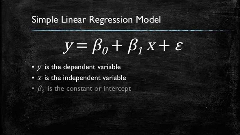
The equation for this linear regression model can be represented as:

y= β0 + β1x + ε

Where:

β0 is the intercept,
β1 is the coefficient of the predictor variable x,
ε is the residual (the difference between the predicted value and the actual value of y).

So, the equation explicitly shows the intercept (β0), the coefficient (β1), and the residuals (ε).

For example, if we have:

Intercept (β0) = 7
Coefficient (β1) = 12
Residual (ε) = 1

Our linear regression equation would be:

y = 7+ 12x + 1

Sure, let’s simplify the explanations:

1. Coefficients: Coefficients are like the helpers in a math problem. In linear regression, they’re just numbers that you multiply with your predictor variables to make predictions about the outcome. They’re like sidekicks helping your main hero (the outcome) along.

2. Intercept: Think of the intercept as the starting point on a journey. In linear regression, it’s the point where your prediction line crosses the y-axis when all your predictors are zero. It’s like the starting point on a treasure map, giving you a clue about where your predictions begin.

3. Residuals: Residuals are the leftovers from your predictions that don’t quite fit perfectly. They’re the difference between what happened and what your model predicted. Picture them as those last few pieces in a puzzle that just don’t fit, no matter how hard you try.

Evaluating Model Performance

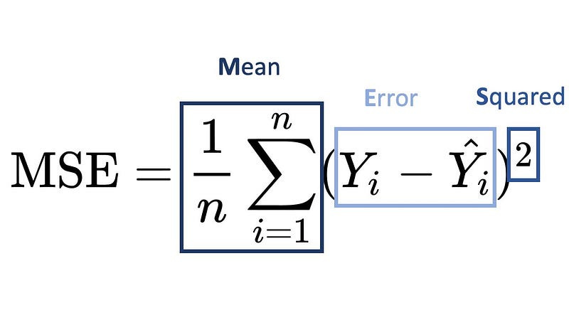
Mean squared error (MSE) defines how big is the error in regression models. Its definition is the average squared difference between the observed and predicted. When MSE equals zero means model has no error. When there is error, its value increases.

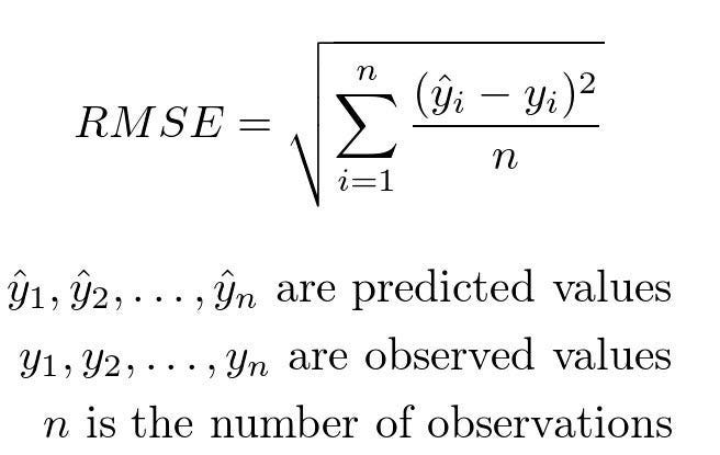
Root mean square error or root mean square deviation is one of the most commonly used measures for evaluating the quality of predictions in regression models. It measures the distance between predictions and true values using Euclidean distance.

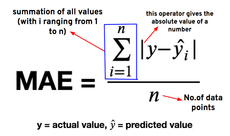
Mean absolute error (MAE) is a popular metric. The MAE score is measured as the average of the absolute error values. It is the difference between the measured value and true value. For example, if a scale states 97 kilos but you know your true weight is 93 pounds, then the scale has an absolute error of 97 kg — 93 kg= 4 kg.

Which one is the best to use as error measurement, this depends on your use case and for robustness to outliers, MAE is less sensitive to outliers compared to MSE and RMSE. In MSE and RMSE, errors are squared before they are averaged, which gives a disproportionately large weight to large errors (outliers). This can skew the overall error metric if your data has many outliers or is highly variable.

Practical Application: How to Implement Linear Regression Using Python or R Programming Language

import numpy as np

class LinearRegression:
    def __init__(self, learning_rate=0.01, n_iterations=1000):
        self.learning_rate = learning_rate
        self.n_iterations = n_iterations
        self.weights = None
        self.bias = None

    def fit(self, X, y):
        n_samples, n_features = X.shape

        self.weights = np.zeros(n_features)
        self.bias = 0

        for _ in range(self.n_iterations):
            # Predicted values
            y_pred = np.dot(X, self.weights) + self.bias

            # Compute gradients
            dw = (1/n_samples) * np.dot(X.T, (y_pred - y))
            db = (1/n_samples) * np.sum(y_pred - y)

            # Update weights and bias
            self.weights -= self.learning_rate * dw
            self.bias -= self.learning_rate * db

    def predict(self, X):
        return np.dot(X, self.weights) + self.bias

def mean_squared_error(y_true, y_pred):
    return np.mean((y_true - y_pred) ** 2)

def root_mean_squared_error(y_true, y_pred):
    return np.sqrt(mean_squared_error(y_true, y_pred))

def mean_absolute_error(y_true, y_pred):
    return np.mean(np.abs(y_true - y_pred))

if __name__ == "__main__":
    np.random.seed(0)
    X = 2 * np.random.rand(100, 1)  
    y = 3 * X + 4 + np.random.randn(100, 1)
    
    # Create and train the model
    model = LinearRegression()
    model.fit(X, y)

    # Predictions
    X_test = np.array([[0.5], [1.5]])
    predictions = model.predict(X_test)
    print("Predictions:", predictions)
    
    # Evaluation
    mse = mean_squared_error(y, model.predict(X))
    rmse = root_mean_squared_error(y, model.predict(X))
    mae = mean_absolute_error(y, model.predict(X))
    print("Mean Squared Error:", mse)
    print("Root Mean Squared Error:", rmse)
    print("Mean Absolute Error:", mae)

Thanks for reading Data Akkadian! This post is public so feel free to share it.